In some of our articles in the past, we learned about different fundamentals of neural networks and deep learning. We saw how to create feed forward neural networks, CNN, and autoencoders using different libraries in R. You can read those from the below links:
Feed-Forward Neural Networks With mxnetR
Anomaly Detection Using H2O Deep Learning
In this article, we will start working on Keras in Python. This is a piece from my new book Hands-on Automated Machine Learning. We will build on this article and take baby steps to master Keras DL through a series of articles focused on deep learning in Python.
Keras is a deep learning library, originally built on Python, that runs over TensorFlow or Theano. It was developed to make DL implementations faster.
We call install Keras using the following command in your operation system’s Command Prompt:
pip install keras
We start by importing the numpy and pandas library for data manipulation. Also, we set a seed that allows us to reproduce the script’s results:
import numpy as np
import pandas as pd
numpy.random.seed(8)
Next, the sequential model and dense layers are imported from keras.models and keras.layers respectively. Keras models are defined as a sequence of layers. The sequential construct allows the user to configure and add layers. The dense layer allows a user to build a fully connected network:
from keras.models import Sequential
from keras.layers import Dense
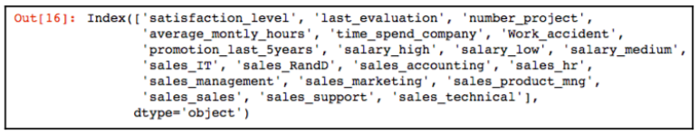
The HR attrition dataset is then loaded, which has 14,999 rows and 10 columns. The salary and sales attributes are one-hot encoded to be used by Keras for building a DL model:
#load hrdataset
hr_data = pd.read_csv('data/hr.csv', header=0)
# split into input (X) and output (Y) variables
data_trnsf = pd.get_dummies(hr_data, columns =['salary', 'sales'])
data_trnsf.columns
X = data_trnsf.drop('left', axis=1)
X.columns
The following is the output from the preceding code:
The dataset is then split with a ratio of 70:30 to train and test the model:
from sklearn.model_selection import train_test_split
X_train, X_test, Y_train, Y_test = train_test_split(X,
data_trnsf.left, test_size=0.3, random_state=42)
Next, we start creating a fully connected neural network by defining a sequential model using three layers. The first layer is the input layer. In this layer, we define the the number of input features using the input_dim argument, the number of neurons, and the activation function. We set the input_dim argument to 20 for the 20 input features we have in our preprocessed dataset X_train. The number of neurons in the first layer is specified to be 12. The target is to predict the employee attrition, which is a binary classification problem. So, we use the rectifier activation function in the first two layers to introduce non-linearity into the model and activate the neurons. The second layer, which is the hidden layer, is configured with 10 neurons. The third layer, which is the output layer, has one neuron with a sigmoid activation function. This ensures that the output is between 0 and 1 for the binary classification task:
# create model
model = Sequential()
model.add(Dense(12, input_dim=20, activation='relu'))
model.add(Dense(10, activation='relu'))
model.add(Dense(1, activation='sigmoid'))
Once we configure the model, the next step is to compile the model. During the compilation, we specify the loss function, the optimizer, and the metrics. Since we are dealing with a two class problem, we specify the loss function as binary_crossentropy. We declare adam as the optimizer to be used for this exercise. The choice of the optimization algorithm is crucial for the model’s excellent performance. The adam optimizer is an extension to a stochastic gradient descent algorithm and is a widely used optimizer:
# Compile model
model.compile(loss='binary_crossentropy', optimizer='adam',
metrics=['accuracy'])
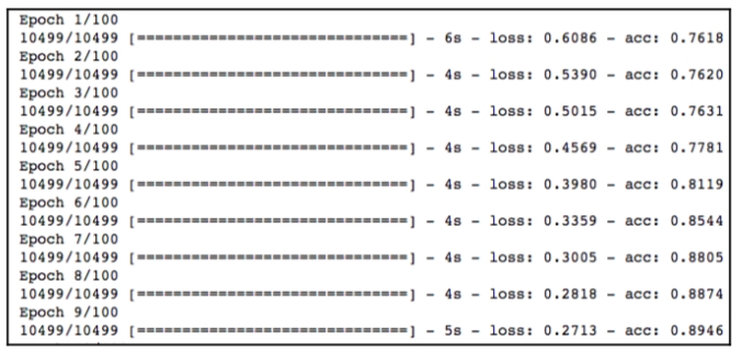
Next, we fit the model to the training set using the fit method. An epoch is used to specify the number of forward and backward passes. The batch_size parameter is used to declare the number of training examples to be used in each epoch. In our example, we specify the number of epochs to be 100 with a batch_size of 10:
# Fit the model
X_train = np.array(X_train)
model.fit(X_train, Y_train, epochs=100, batch_size=10)
Once we execute the preceding code snippet, the execution starts and we can see the progress, as in the following screenshot. The processing stops once it reaches the number of epochs that is specified in the model’s fit method:
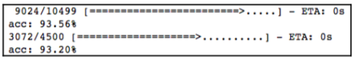
The final step is to evaluate the model. We specified accuracy earlier in the evaluation metrics. At the final step, we retrieve the model’s accuracy using the following code snippet:
# evaluate the model
scores = model.evaluate(X_train, Y_train)
print("%s: %.4f%%" % (model.metrics_names[1], scores[1]*100))
X_test = np.array(X_test)
scores = model.evaluate(X_test, Y_test)
print("%s: %.4f%%" % (model.metrics_names[1], scores[1]*100))
The following result shows the model accuracy to be 93.56% and test accuracy to be 93.20%, which is a pretty good result. We might get slightly different results than those depicted as per the seed: