Interactive Topic Modeling Using Python

Mining information out of text data is one of the most critical use cases that every enterprise is undertaking. There are a lot of unstructured data that gets generated every day, which can provide a ton of information. Unstructured data can be in any form of natural language – audio, video, or written transcripts – and executives are curious to see the value that can be generated out of this unstructured data. The use cases in and around audio and video data might not be attractive to every enterprise, but the information out of text data is. It might be analyzing the contents of an email to identify whether it is a potential phishing email, analyzing communication between customers and sales reps to identify the likelyhood of a deal closure, or just understanding the sentiment of our customers towards our organization. Written communications remain the ideal medium of communication and mining that data provides a plethora of information.

In this post, we will look at topic modeling, one of the most used techniques to derive insights out of text data. In a nutshell, topic modeling helps categorize various sentences into various topics. This assists in understanding the significant themes in multiple texts and proves useful for sorting various texts into specific categories. You can imagine this as tagging various files into different folders but done automatically by a machine learning model.

I have previous written some pieces on preprocessing text, creating document clusters, and classifying different articles/text using R. These pieces are going to give you some idea on how to start with clean text and get started with text data. This piece will focus on creating topic models in Python and have an interactive result viewer that can provide you information on the model results and guide you on effectively judging the accuracy of your topic models.

The first step is to load various libraries for reading the files, text processing, and visualization. We will be using NLTK (Natual Language Toolkit) for this exercise. The NLTK package is a leading library for building applications around Natural Language data. It provides various text processing capabilities, such as easy to use text preprocessors, and text-based model techniques, like document classification, named entity recognition, and much more. There are other new libraries such as spaCy in Python that we would explore in future articles.

import os

import numpy as np

import pandas as pd

import re

import string

# NLTK Stop words

import nltk

from nltk.corpus import stopwords

from nltk import TweetTokenizer

from nltk.stem import WordNetLemmatizer

# Gensim

import gensim

import gensim.corpora as corpora

from gensim.utils import simple_preprocess

from gensim.models import CoherenceModel

# Plots

import pyLDAvis

import pyLDAvis.gensim  # don't skip this

import matplotlib.pyplot as plt

%matplotlib inline

The next step is to read the text files. The following code reads all the files in a folder and does some necessary text clean up, such as removing newline characters, quotes, and extra spaces.

path = '\zone\text_mining\document_clustering'

fileList = os.listdir(path)

for i in fileList:

    file = open(os.path.join(path+'/'+ i), 'r')

data = file.readlines()

data = [re.sub('\s+',' ', sent) for sent in data]

data = [re.sub('\'', '', sent) for sent in data]

data = [x for x in data if x != ' ']

print(data)

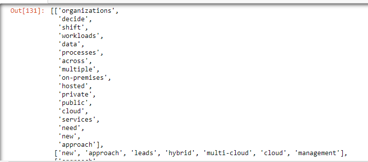
Now, we need to create tokens out of the text. Tokens can be loosely defined as words, but technically it is a sequence of characters that are grouped as a semantic unit. The nltk.sent_tokenize method splits the document/text into sentences. Then each sentence is tokenized in words using word_tokenize.

When we create tokens, there are certain words like prepositions and punctuations (the, an, in, etc.) that are commonly used in every English sentence. These words don’t add much value in text analysis or modeling tasks. These are just redundant pieces of information that can be removed. These words are technically termed stopwords, and are made available as a pre-defined list for us to use directly. We can add custom stopwords to the list that we think are not valuable in our text and not available as a part of the standard stopword list. The following code demonstrates the process to create tokens for every sentence after removing the stopwords.

val = ','.join(data)

stopwords_punct = set(stopwords.words('english')).union(string.punctuation).union('-')

sentences = nltk.sent_tokenize(val)

sents_stopwords_rm = []

for sent in sentences:

    sents_stopwords_rm.append(' '.join(w for w in nltk.word_tokenize(sent) if w.lower() not in stopwords_punct))

data_tokens_no_stopwords = [nltk.word_tokenize(t) for t in sents_stopwords_rm]

data_tokens_no_stopwords

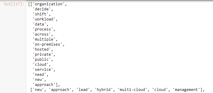
Once we have the tokens, we need to stem them to their root form. For example, ‘describing’ and ‘described’ are the present and past tense of the word ‘describe.’ The objective of this topic modeling exercise is to categorize words into various topics. So, instead of preserving the conjugated forms of a word, we need to bring them down to their root form that increases the strength of the words in the document. Stemming and Lemmatized are two favorite ways of reducing the derived words to their root form. The significant difference between these is that stemming can often create non-existent words, whereas lemmas are actual words. In the below code snippet, we use WordNetLemmatizer to create lemmas for the tokens that we created earlier.

wordnet_lemmatizer = WordNetLemmatizer()

data_lemmatized = []

for w in data_tokens_no_stopwords:

 data_lemmatized.append([word for word in map(wordnet_lemmatizer.lemmatize, w)])

data_lemmatized

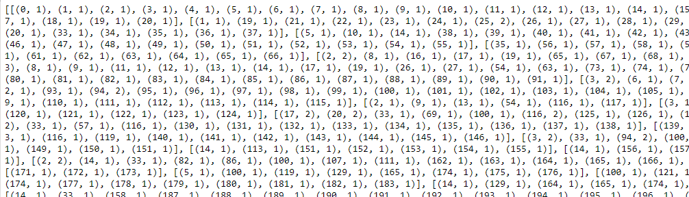
Next, we need to generate a document term frequency matrix to create an LDA model. The document term frequency matrix counts how frequently a term appears in a document. For that, first, we create a dictionary of documents using the corpora.Dictionary method.

The Dictionary() function traverses each document and assigns a unique id to each unique token along with their counts.

Next, the dictionary is converted into a bag-of-words using the doc2bow method. The result is a list of vectors equal to the number of documents. Each document vector has a series of tuples with token id and token frequency pair.

# Create Corpus

dictionary = corpora.Dictionary(data_lemmatized)

corpus = [dictionary.doc2bow(text) for text in data_lemmatized]

print(corpus)

Now that we have the data in the format required by the LDA Model, we can invoke the ldamodel from the gensim package with our data and other required parameters.

# Build LDA model

ldamodel = gensim.models.ldamodel.LdaModel(corpus=corpus,

                                           id2word=dictionary,

                                           num_topics=5,

                                           passes=10,

                                           alpha='auto',

                                           per_word_topics=True)

The LdaModel class and its parameters are described in detail in the gensim documentation. The following is a brief description of the parameters that are used in our model.

• corpus  – The input is the doc2bow bag of words vector that was prepared in the previous step.
• id2word – This requires the dictionary that was prepared in the previous step.
• num_topics – The number of latent topics that are to be extracted from the training corpus.
• passes – Number of passes through the corpus during training.
• per_word_topics – If True, the model also computes a list of topics, sorted in descending order of most likely topics for each word.

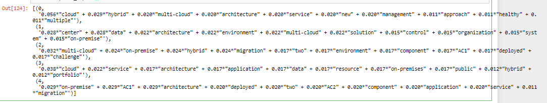
Next, we print the keywords along with thier weightages in each topic using the ldamodel.print_topics() method:

# Print the keywords and thier weightages in each topic

ldamodel.print_topics()

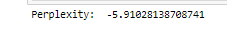
We can also judge the accuracy of the topic model by calculating the perplexity metric. It a measure of how good the model is. The lower the value, better is the model.

print('Perplexity: ', ldamodel.log_perplexity(corpus))

Next, we can visualize the LDA output using the pyLDAvis plot. It is an interactive plot, where each bubble represents a topic. The larger the bubble size, the more prevailing that topic is. A good topic model will have large non-overlapping bubbles in the chart. The bar plot one right-hand side of the screenshot shows the frequency of the terms in the topic, out of the total term frequency in the documents. From the following chart, we can infer that we have created a good topic model.

Now that we are ready with the topic model, we can assign and tag each statement with its most relevant topic number. The following code snippet can simply do that for you. I noticed this wonderful snippet from this article.

def format_topics_sentences(ldamodel=None, corpus=corpus, texts=data):

    # Init output

    sent_topics_df = pd.DataFrame()

    # Get main topic in each document

    for i, row_list in enumerate(ldamodel[corpus]):

        row = row_list[0] if ldamodel.per_word_topics else row_list

        # print(row)

        row = sorted(row, key=lambda x: (x[1]), reverse=True)

        # Get the Dominant topic, Perc Contribution and Keywords for each document

        for j, (topic_num, prop_topic) in enumerate(row):

            if j == 0:  # => dominant topic

                wp = ldamodel.show_topic(topic_num)

                topic_keywords = ", ".join([word for word, prop in wp])

                sent_topics_df = sent_topics_df.append(pd.Series([int(topic_num), round(prop_topic,4), topic_keywords]), ignore_index=True)

            else:

                break

    sent_topics_df.columns = ['Dominant_Topic', 'Perc_Contribution', 'Topic_Keywords']

    # Add original text to the end of the output

    contents = pd.Series(texts)

    sent_topics_df = pd.concat([sent_topics_df, contents], axis=1)

    return(sent_topics_df)

df_topic_sents_keywords = format_topics_sentences(ldamodel=ldamodel, corpus=corpus, texts=data)

# Format

df_dominant_topic = df_topic_sents_keywords.reset_index()

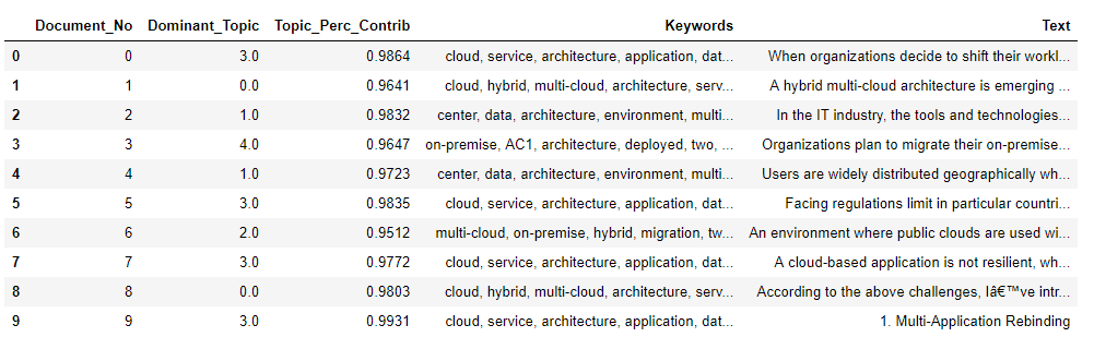
df_dominant_topic.columns = ['Document_No', 'Dominant_Topic', 'Topic_Perc_Contrib', 'Keywords', 'Text']

# Show

df_dominant_topic.head(10)

The following table displays the document along with the common topic, the keywords, and the percentage contribution of the topic in the document text.

You can find the code along with the data on my GitHub repo.