This is the second article in our series — Data Science Start-Ups in Focus — where we’ll deep dive into the start-ups in the area of data science and analytics to learn from their unique perspectives in the field. The goal here is to introduce readers to some new helpful platforms & tools, to show companies doing interesting things related to Machine Learning & the Big Data space. The first part of the series shined the spotlight on BigML. If you missed this issue, check it out.
Introduction to H2O.ai
This month we focus on H2O.ai, an AI platform whose mission is to bring AI to enterprises. H2O.ai software is built on Java, Python, and R. Its purpose is to optimize Machine Learning for Big Data and deliver business transformation through AI. It’s offered as open source to drive contribution.
Features that stands out on this platform are:
1) Big Data Friendly – Organizations can use all of their data in real-time for better predictions with H2O’s fast in-memory distributed parallel processing capabilities. Check out the performance benchmark video on how PayPal trains models in 10 min and scores data in 5 min using H2O and Hadoop, compared to other flavors of R and Databases which takes days to complete the same model.
2) Open Source Development and Support – Open source drives contribution, and H2O believes in the community power. So, H2O libraries are present almost for all the best brands of open source Big Data development Platforms.
3) Production Deployment made easy – Using H2O, a developer need not worry about the variation in the development platform and production environment. H2O models once created can be utilized and deployed like any Standard Java Object. H2O models are compiled into POJO (Plain Old Java Files) or a MOJO (Model Object Optimized) format which can easily embed in any Java environment.
4) Machine Learning platform for all – The beauty of H2O is that its algorithms can be utilized by:
- Business analysts and statisticians who are not familiar with programming languages using its Flow Web UI (User Interface).
- Developers who know any of the widely used programming languages – Java, R, Python, Spark
H2O has seen a high surge of users in 2016, and the count only keeps rising. It becomes apparent when one hangs on Kaggle’s Machine Learning competitions as well as the discussion forum just how important H2O algorithms are to data scientist.
H2O.ai in Action
For the rest of this article, we’ll focus on using H2O and R to solving the classic problem of credit scoring using this German Credit Dataset. The German Credit Data contains data on 20 variables and the classification whether an applicant is considered a Good or a Bad credit risk for 1000 loan applicants. You can retrieve the dataset from this GitHub repo.
First off, you’ll need to install H2O. I have detailed this process in my previous article Anomaly Detection using H2O Deep Learning which you can refer to for the details.
Alright, we are now ready to explore H2O… let’s sail off into the deep blue waters.
Let’s first import the data into H2O cluster using the below code snippet. You can also use h2o.uploadFile and as.h2o to load data. The difference between these three is described in our previous article.
library(h2o)
h2o.init()
data<-h2o.importFile("F:/git/credit_scoring/german_credit.csv")
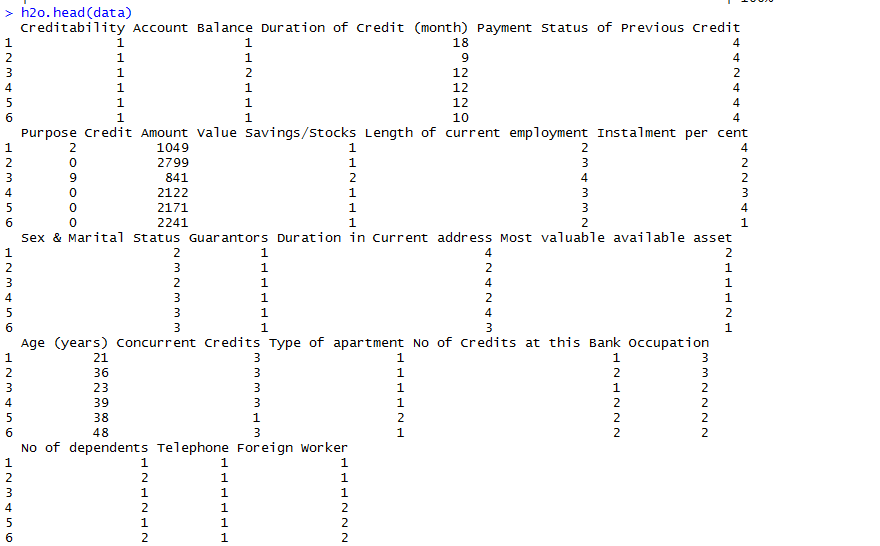
Next, we use h2o.head(data) to view the first few rows of an H2OFrame object. It comes in handy for inspecting the data and analyzing how the data looks after import. The h2o.head() is an optimized version of the R’s head() to work on the H2OFrame object.
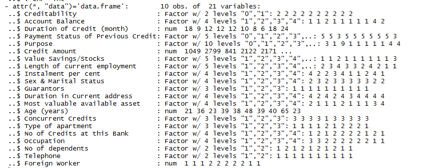
Following that, we describe the aggregated information about the data using h2o.describe(data). The result contains the information about data types, min and max values, the missing values, count of zeros, the standard deviation of values for each column. It also displays the number of levels for the categorical/factor columns.
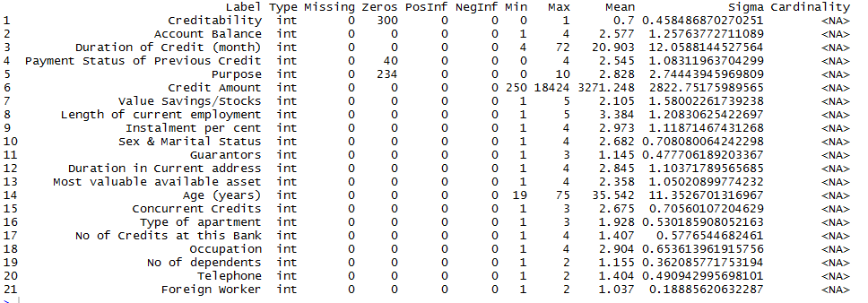
From the above result screenshot, we observe that there are some variables like Creditability and Payment Status of Previous Credit which should be of type factor/enum(in H2O). So, we type cast them using the below code. h2o.asfactor() converts H2O Data to factors.
### Convert Numeric to Categorical ###
to_factors <- c(1,2,4,5,7,8,9,10,11,12,13,15,16,17,18,19,20)
for(i in to_factors) data[,i] <- h2o.asfactor(data[,i])
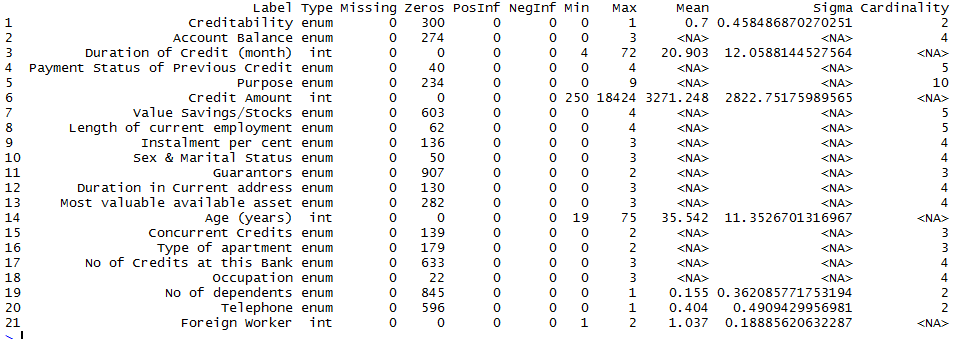
Again, we describe the data using h2o.describe(data) function. This time we see the data type as per our expectation and also the number of levels of each factor, i.e. Cardinality available for all enum variables.
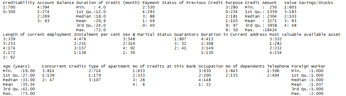
h2o.summary(data) is another useful summary function. It displays the minimum, 1st quartile, median, mean, 3rd quartile and maximum for each numeric column, and the levels and category counts of the levels in each categorical column.
Next, we come to another handy function h2o.str(data) that displays the structure of an H2OFrame object.
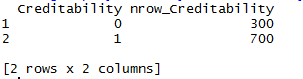
We now check the number of data rows available to create the classification model for each class of the target variable. This also provides us with information useful for understanding whether the data set is unbalanced. Modeling on unbalanced data set introduces error on the prediction and is more biased towards the class with more of records. So, generally, in such cases data is sampled again to be balanced or adjust the class weights during model creation. Not all algorithms support class weights and so we need to check algorithm definitions to find out.
We can use h2o.group_by function to count the number of rows for each target class as shown in below code.
h2o.group_by(data, by="Creditability",nrow("Creditability"))
Another useful function from H2O is h2o.log which can be used for logarithmic transformations over the H2O data.
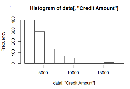
Let’s plot the histogram of the Credit Column data using h2o.hist(data[,"Credit Amount"]). We can alternatively use positional notion to refer the column like h2o.hist(data[,6])
Apply the log function to the Credit Amount, store it in a new variable credit_amount_trnsf and plot the histogram.
data$credit_amount_trnsf <- h2o.log(data[,"Credit Amount"])
h2o.hist(data$credit_amount_trnsf)
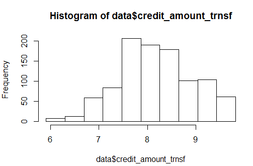
After the log transformation, data looks somewhat close to normal. Let’s stick to it for now. To create a supervised model such as classification, we need to annotate the target and input predictors so that it can make predictions.
For that, let us define the column Creditability (Good/Bad credit) as the Target for modeling.
target <- "Creditability"
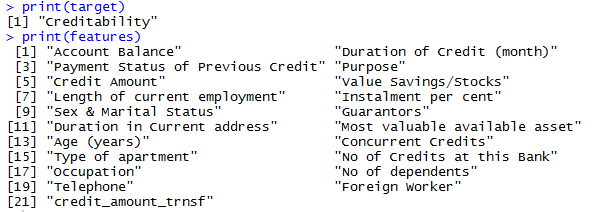
Now that we have assigned Creditability as a Target, let’s remove it from the column list and assign remaining to a new variable called “features” which serves as a list of input predictors.
To train and test the model, let’s partition the data into training(60%) and test set(40%). Setting a seed will guarantee reproducibility.
Now that we have prepared our data, let’s build a Generalized Linear Model(glm) using the h2o.glm function. We will go into more detail about this in future articles. You can run the below code snippet to create a GLM model and can refer to H2O’s GLM Docs page for more information.
glm_model1 <- h2o.glm(x = features,
y = target,
training_frame = credit_train,
model_id = "glm_model1",
family = "binomial")
Once the model building is completed successfully, you can view the model build summary using print(summary(glm_model1)). The model build summary displays information about the fields, build settings, and model estimation process.
The next important step is to evaluate whether the model can be as accurate on new data as it is in the training data. For this step, we’d already held out some portion of the data as a test data. Use h2o.performance to evaluate the model performance on the held-out test dataset. Usually, to validate the model on test data, we first do the predictions using predict methods in R and then compute the metrics using other functions. However, using h2o packages, we can just wield the h2o.performance method to validate the performance of the test data. The result has all the performance measures that can be computed for that model. Track and choose the best metrics you want to evaluate your model. This is a cool feature and saves a lot of time!
perf_obj <- h2o.performance(glm_model1, newdata = credit_test)
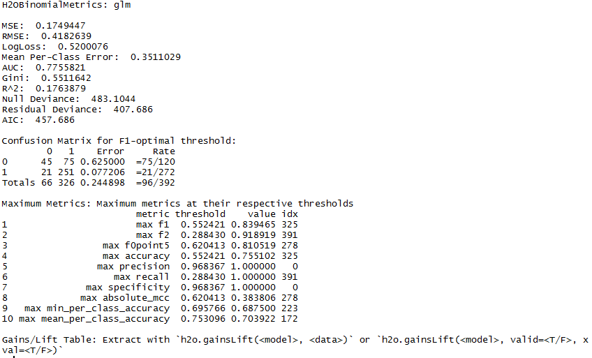
Alternatively, you can use the H2O Model metric accessor functions to print out only the evaluation metric of your choice. The complete list of these functions is available here. For our example, let’s view the accuracy of the model at 0.95 thresheld.
h2o.accuracy(perf_obj,0.944485973651485)
Use the h2o.predict method to do predictions on the new data. For this example, we stick to the predictions on the same test data set.
pred_creditability <- h2o.predict(glm_model1,credit_test)
pred_creditability
As always, this illustration was just a drop of water that H2O offers. You can get started by following the H2O’s documentation. The material is quite extensive and useful to start with. Other than that, if you want to understand deeply and gets your hands dirty with machine learning and AI using H2O.ai, you should enroll for the Enterprise AI course taught by our MVB Ajit Jaokar and in partnership with H2O.ai.
